Elmera Azadpour - Binary Logistic Regression

To access data, html and Rmd/qmd files:

the palmetto data can be found in the data folder of this repo; the Rmd and html files, denoted as a2-task2, can be found in the src folder
the qmd format can be found here

Load packages

library(tidyverse)
library(here)
library(GGally)
library(broom)
library(jtools)
library(kableExtra)

Read in data

palmetto <- read_csv(here("posts", "2021-02-23-blrpalmetto", "palmetto.csv"), 
                     col_types = cols(.default = "c")) %>%
  mutate(height = as.numeric(height)) %>% 
  mutate(species_name = case_when(
    species == 1 ~ "Serenoa repens", 
    species == 2 ~ "Sabal etonia")) %>% 
  mutate(site_name = case_when(
    site == 1 ~ "Copse Road", 
    site == 2 ~ "Ridge Road",
    site == 3 ~ "WSP2",
    site == 4 ~ "WS30",
    site == 5 ~ "WSP1",
    site == 6 ~ "Red Hill"))  %>% 
  mutate(width = as.integer(width)) %>% 
  mutate(length = as.integer(length)) %>% 
  mutate(green_lvs = as.integer(green_lvs))

Data exploration between species 1 (Serenoa repens) and species 2 (Sabal etonia).

ggplot(palmetto,
       aes(x = species_name, y = height)) +
  geom_boxplot(aes(fill = species_name)) +
  facet_wrap(~ site_name) +
  labs(x = "Species", y = "Canopy height (cm)") +
  scale_fill_discrete(name = "Species") +
  theme_light() +
 theme(legend.position = "top")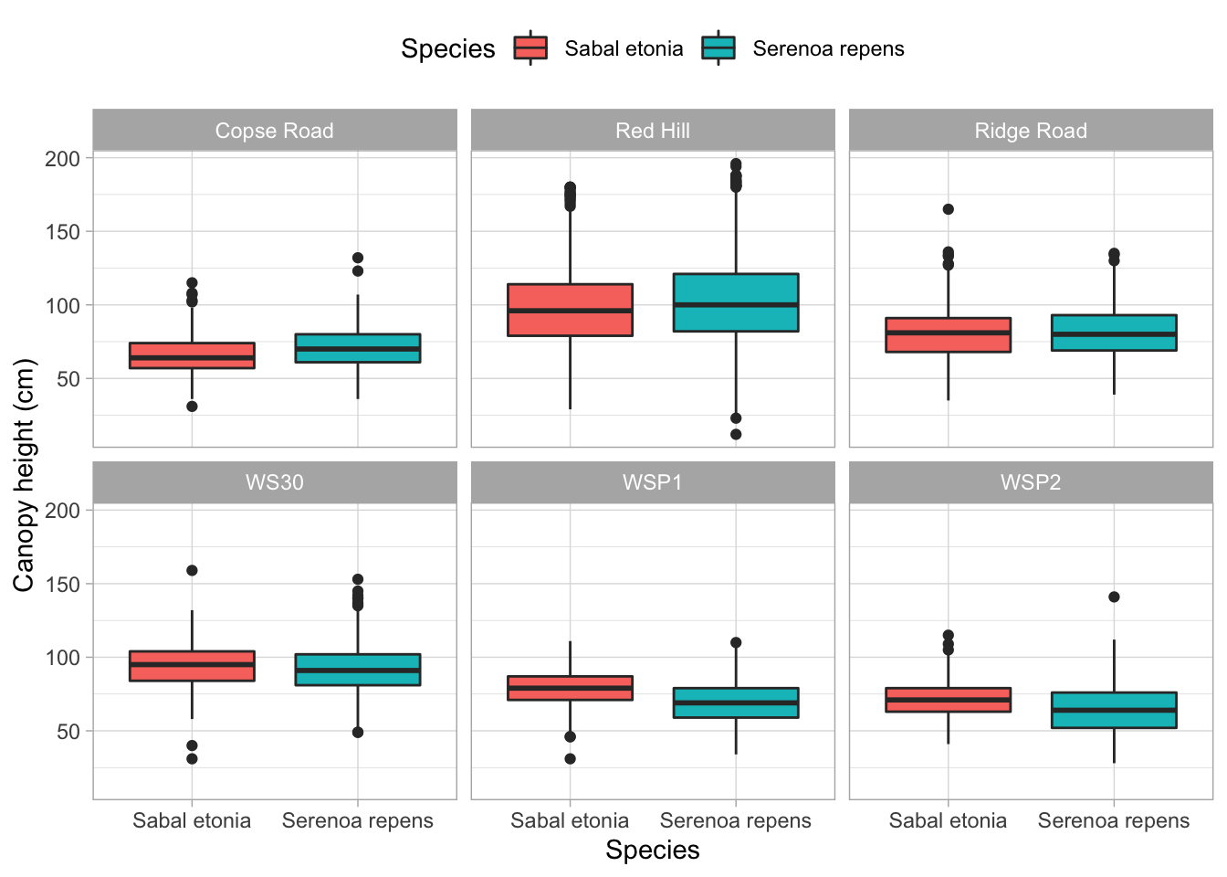

**Figure 1**. Species (Sabal etonia and Sernoa repens) vs canopy height (cm) by study site. Generally Sabal etonia tends to have higher canopy height than Serenoa repens across the sites.

Graph 2

ggplot(palmetto, aes(x = width, y = length)) +
  geom_point(aes(color = species_name)) +
  theme_minimal() +
  labs(x = "Canopy width (cm)", y = "Canopy height (cm)") +
  scale_color_discrete(name = "Species") +
 theme(legend.position = "top")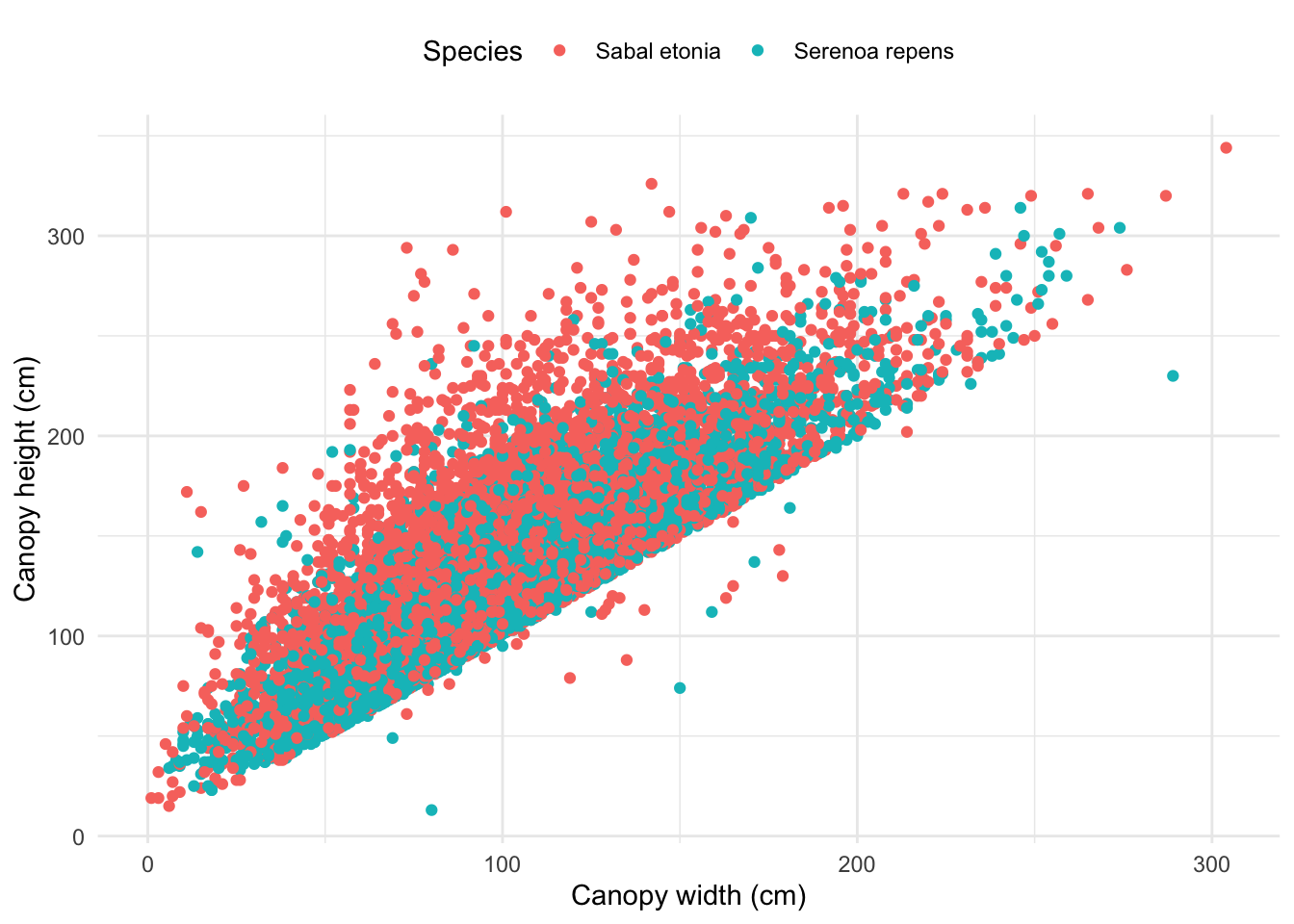

**Figure 2**. Canopy width (cm) vs canopy height (cm) for both species (Sabal etonia and Serenoa repens). Trend indicates Sabal etonia trees tend to have more lower capopy width and higher canopy height as compared to Serenoa repens, however still lots of spread in the data.

Binary logistic regression using plant height, canopy length, canopy width and green leaves as predictor variables to understand how they relate to probability of a plant being Serenoa repens or Sabal etonia

palmetto_blr_ds <- palmetto %>% 
  mutate(species_name = fct_drop(species_name)) %>% 
  select(species_name, height, length, width, green_lvs) 
  
palmetto_blr <- glm(species_name ~ height + length + width + green_lvs ,
                            data = palmetto_blr_ds, 
                            family = "binomial")

Look at outcome of blr model

palmetto_blr #


Call:  glm(formula = species_name ~ height + length + width + green_lvs, 
    family = "binomial", data = palmetto_blr_ds)

Coefficients:
(Intercept)       height       length        width    green_lvs  
   -3.09204      0.02930     -0.04571     -0.03927      1.89280  

Degrees of Freedom: 12266 Total (i.e. Null);  12262 Residual
  (193 observations deleted due to missingness)
Null Deviance:      17010 
Residual Deviance: 5166     AIC: 5176

summary(palmetto_blr)


Call:
glm(formula = species_name ~ height + length + width + green_lvs, 
    family = "binomial", data = palmetto_blr_ds)

Deviance Residuals: 
    Min       1Q   Median       3Q      Max  
-4.7821  -0.2637  -0.0055   0.1715   3.3631  

Coefficients:
             Estimate Std. Error z value Pr(>|z|)    
(Intercept) -3.092041   0.141270  -21.89   <2e-16 ***
height       0.029304   0.002311   12.68   <2e-16 ***
length      -0.045713   0.001872  -24.41   <2e-16 ***
width       -0.039266   0.002102  -18.68   <2e-16 ***
green_lvs    1.892804   0.038591   49.05   <2e-16 ***
---
Signif. codes:  0 '***' 0.001 '**' 0.01 '*' 0.05 '.' 0.1 ' ' 1

(Dispersion parameter for binomial family taken to be 1)

    Null deviance: 17005.5  on 12266  degrees of freedom
Residual deviance:  5166.1  on 12262  degrees of freedom
  (193 observations deleted due to missingness)
AIC: 5176.1

Number of Fisher Scoring iterations: 7

# We can use the broom::tidy() function to get the model outputs in nice data frame format:
palmetto_blr_tidy <- broom::tidy(palmetto_blr)

# Get the intercept: 
palmetto_int <- palmetto_blr_tidy$estimate[1]
palmetto_int

[1] -3.092041

# Then to get the  coefficient:
palmetto_coef <- palmetto_blr_tidy$estimate[2]
palmetto_coef

[1] 0.02930385

#What about getting some other model information (degrees of freedom, F-statistic, p-value, etc.)?
#Many of these statistical outcomes can be accessed more easily using broom::glance().
# Metrics at a glance: 
palmetto_lm_out <- broom::glance(palmetto_blr)
palmetto_lm_out

# A tibble: 1 × 8
  null.deviance df.null logLik   AIC   BIC deviance df.residual  nobs
          <dbl>   <int>  <dbl> <dbl> <dbl>    <dbl>       <int> <int>
1        17006.   12266 -2583. 5176. 5213.    5166.       12262 12267

## tidy model table output
palmetto_blr_tidy %>% 
  kable(col.names = c("Term",
                      "Estimate",
                      "St Error",
                      "t-statistic",
                      "p-value")) %>% 
  kable_styling(full_width = FALSE)

Term	Estimate	St Error	t-statistic
(Intercept)	-3.0920409	0.1412703	-21.88740
height	0.0293039	0.0023114	12.67770
length	-0.0457129	0.0018724	-24.41353
width	-0.0392659	0.0021022	-18.67885
green_lvs	1.8928041	0.0385905	49.04843

What does model output tell us? Output tells us that probabiliy of Serenoa repens species because its “1” in the levels. So we expect on average, that as canopy height increases, the odds of the species being Serenoa repens increases. With an increase in canopy length, the odds of the species being Serenoa repens decreases on average. Similarly with width, we expect that as canopy width increases, the odds of the species being Serenoa repens decreases. Lastly, on average as count of green leaves increases, we expect the odds of the species being Serenoa repens increases.

Evaluates how successfully this model would “classify” a plant as the correct species, using a 50% cutoff (e.g. if the probability is >=50% that it is species A, then it would be classified as species A)

palmetto_blr_fitted <- palmetto_blr %>% 
  broom::augment(type.predict = "response") %>% 
  mutate(classification = case_when(.fitted >=0.50 ~ "Serenoa repens", 
      TRUE ~ "Sabal etonia")) 
  

palmetto_table <- palmetto_blr_fitted %>% 
  select(species_name, .fitted, classification) %>% 
  mutate(correct = case_when(
      species_name == "Serenoa repens" & classification == "Serenoa repens" ~ "correct",
      species_name == "Sabal etonia" & classification == "Sabal etonia" ~ "correct",
      TRUE ~ "incorrect"))
  
  
palmetto_summary_table <- palmetto_table %>% 
  group_by(species_name, correct) %>% 
  summarise(count = n()) %>% 
  mutate(percentcorrect = (count / sum(count)*100))

`summarise()` has grouped output by 'species_name'. You can override using the
`.groups` argument.

palmetto_summary_table %>%  
  kable(col.names = c("Species name",
                      "Correct or incorrect model classification?",
                      "Count",
                      "% Correctly classified"), 
        caption = "**Table 1**: summary statistics binary logistic regression analysis on palmetto dataset including species: Serenoa repens & Sabal etonia (data source: Abrahamson, W.G. 2019. Survival, growth and biomass estimates of two dominant palmetto species of south-central Florida from 1981 - 2017, ongoing at 5-year)") %>% 
  kable_styling(full_width = FALSE)

**Table 1**: summary statistics binary logistic regression analysis on palmetto dataset including species: Serenoa repens & Sabal etonia (data source: Abrahamson, W.G. 2019. Survival, growth and biomass estimates of two dominant palmetto species of south-central Florida from 1981 - 2017, ongoing at 5-year)
Species name	Correct or incorrect model classification?	Count	% Correctly classified
Sabal etonia	correct	5688	92.412673
Sabal etonia	incorrect	467	7.587327
Serenoa repens	correct	5541	90.657723
Serenoa repens	incorrect	571	9.342277