library(tidyverse)
library(here)
library(broom)
library(effsize)
library(janitor)
library(kableExtra)Load Packages:
To access data, html and Rmd/qmd files:
Read in sea turtles data (source: Environmental Data Initiative)
sea_turtles <- read_csv(here("posts", "2021-03-31-two-sample-t-test", "sharkbay_sea_turtles.csv"))
sea_turtles_clean <- sea_turtles %>%
  dplyr::select(species, length, width, burr)
Exploratory visualization
ggplot(sea_turtles_clean, aes(x = length,
                              y= width)) +
  geom_point() +
  theme_minimal()+
  labs(x ="Curved carapace length at midline (cm)",
  y = "Curved carapace width at widest point (cm)")
Warning: Removed 1 rows containing missing values (geom_point).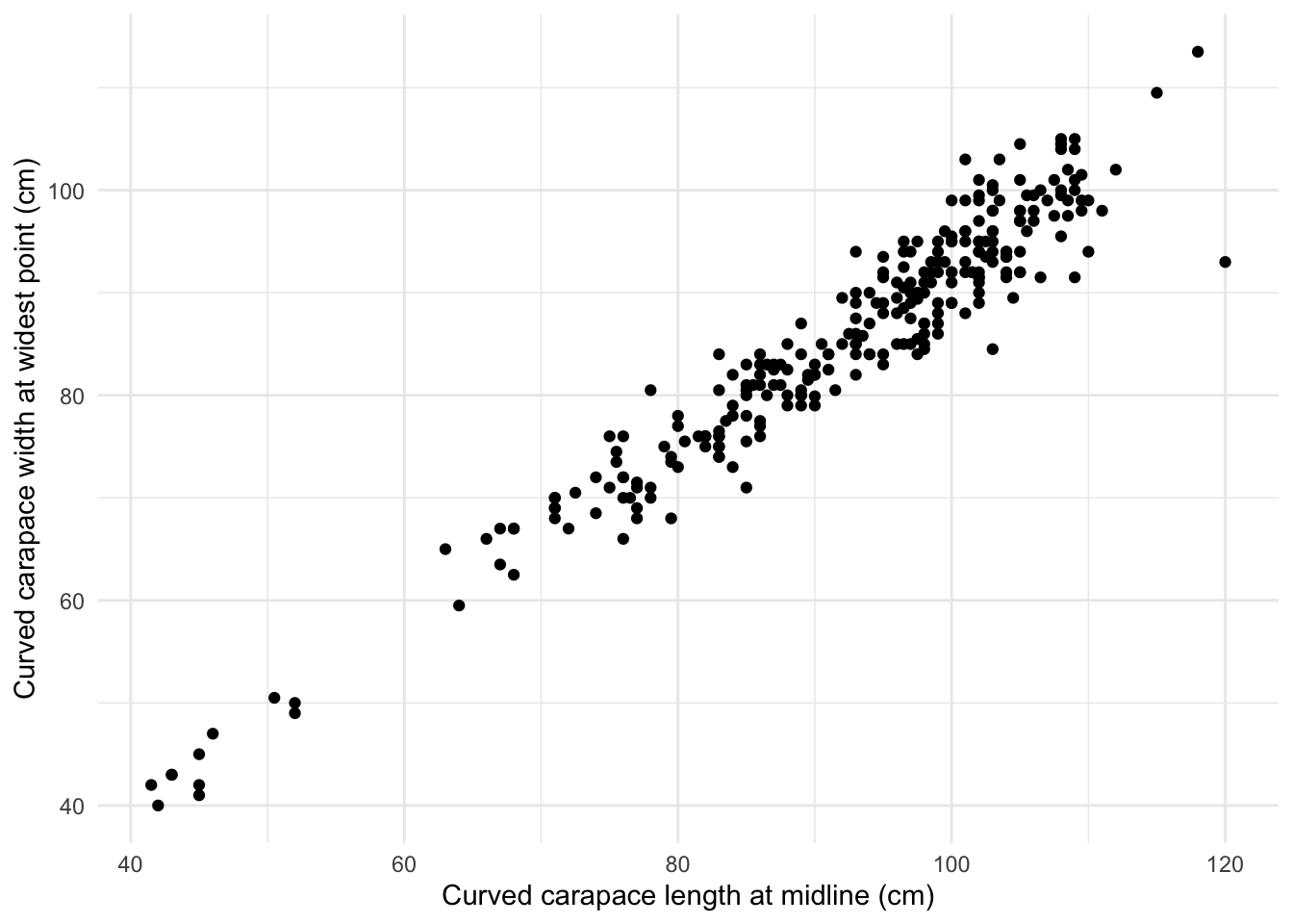
Linear Regression
## linear regression
turtles_lm <- lm(length ~ width, data = sea_turtles_clean)

# Return the complete overview:
summary(turtles_lm)
Call:
lm(formula = length ~ width, data = sea_turtles_clean)

Residuals:
     Min       1Q   Median       3Q      Max
-10.1332  -2.6294   0.0433   2.4164  19.6729

Coefficients:
            Estimate Std. Error t value Pr(>|t|)
(Intercept) -0.16968    1.50479  -0.113     0.91
width        1.08061    0.01749  61.775   <2e-16 ***
---
Signif. codes:  0 '***' 0.001 '**' 0.01 '*' 0.05 '.' 0.1 ' ' 1

Residual standard error: 3.802 on 280 degrees of freedom
  (1 observation deleted due to missingness)
Multiple R-squared:  0.9316,    Adjusted R-squared:  0.9314
F-statistic:  3816 on 1 and 280 DF,  p-value: < 2.2e-16
# We can use the broom::tidy() function to get the model outputs in nice data frame format:
turtles_lm_tidy <- broom::tidy(turtles_lm)
# Get the intercept:
turtles_int <- turtles_lm_tidy$estimate[1]
turtles_int[1] -0.1696804# Then to get the flipper_length coefficient:
turtles_coef <- turtles_lm_tidy$estimate[2]
turtles_coef[1] 1.080611#What about getting some other model information (degrees of freedom, F-statistic, p-value, etc.)?
#Many of these statistical outcomes can be accessed more easily using broom::glance().
# Metrics at a glance:
turtles_lm_out <- broom::glance(turtles_lm)
turtles_lm_out# A tibble: 1 × 12
r.squared adj.r.squ…¹ sigma stati…² p.value df logLik AIC BIC devia…³
<dbl> <dbl> <dbl> <dbl> <dbl> <dbl> <dbl> <dbl> <dbl> <dbl>
1 0.932 0.931 3.80 3816. 3.66e-165 1 -776. 1558. 1568. 4048.
# … with 2 more variables: df.residual <int>, nobs <int>, and abbreviated
# variable names ¹adj.r.squared, ²statistic, ³deviance
# ℹ Use `colnames()` to see all variable names# Explore model assumptions
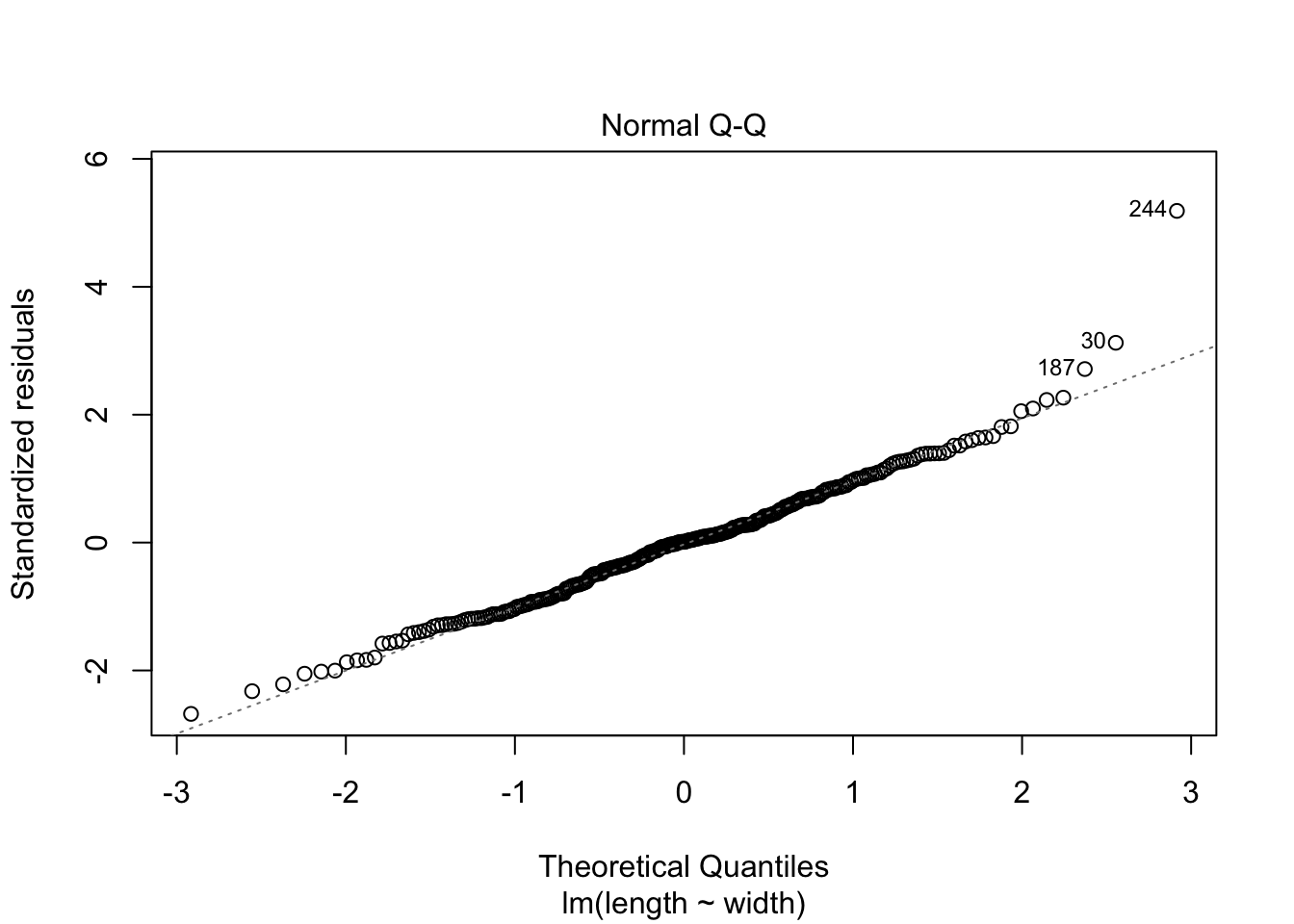
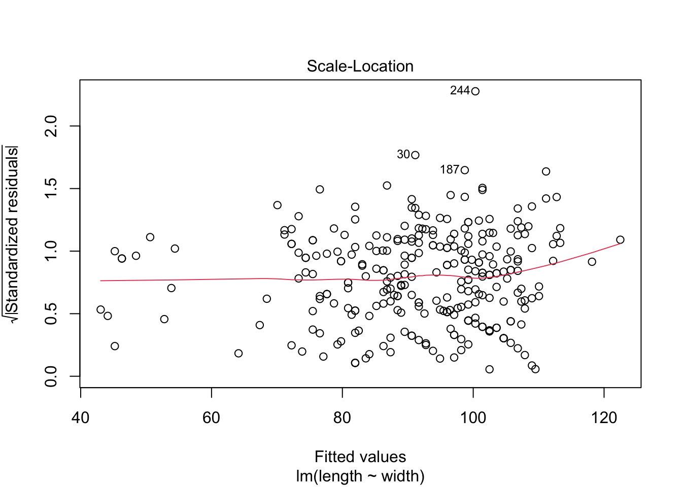
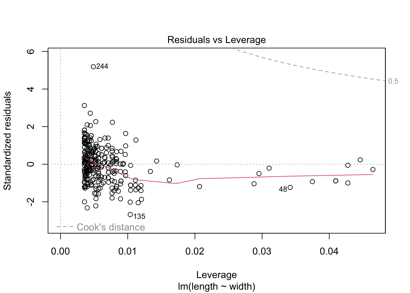
plot(turtles_lm)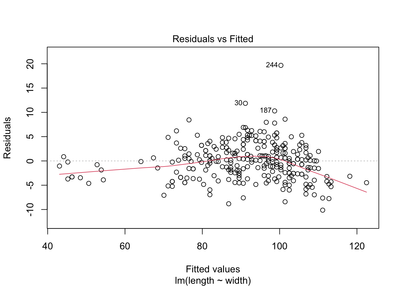
# Pearson’s r
turtles_cor <- cor.test(sea_turtles_clean$length, sea_turtles_clean$width)
turtles_cor
    Pearson's product-moment correlation

data:  sea_turtles_clean$length and sea_turtles_clean$width
t = 61.775, df = 280, p-value < 2.2e-16
alternative hypothesis: true correlation is not equal to 0
95 percent confidence interval:
 0.9562175 0.9723919
sample estimates:
      cor
0.9652165
Regression summary of sea turtle curved carapace length and width at midline (cm).
- Simple linear regression was used to explore the relationship between sea turtles curved carapace length at midline (cm) and curved carapace width at widest point (cm) across two sea turtle species: green or loggerhead. A significant regression model was found (\(\beta\) = 1.081, F(1,280) = 3816.1, p < 0.001) with an R2 of 0.932.
Comparing carapace lengths between green and loggerhead turtles
## Lets just look at the raw data
#ggplot(data = sea_turtles_clean, aes(x = species, y = length)) + geom_boxplot(aes(col=species))
# not very different..

# Histograms
ggplot(data = sea_turtles_clean, aes(x = length)) +
  geom_histogram(bins = 15) +
  facet_wrap(~species, scales = "free")
Warning: Removed 1 rows containing non-finite values (stat_bin).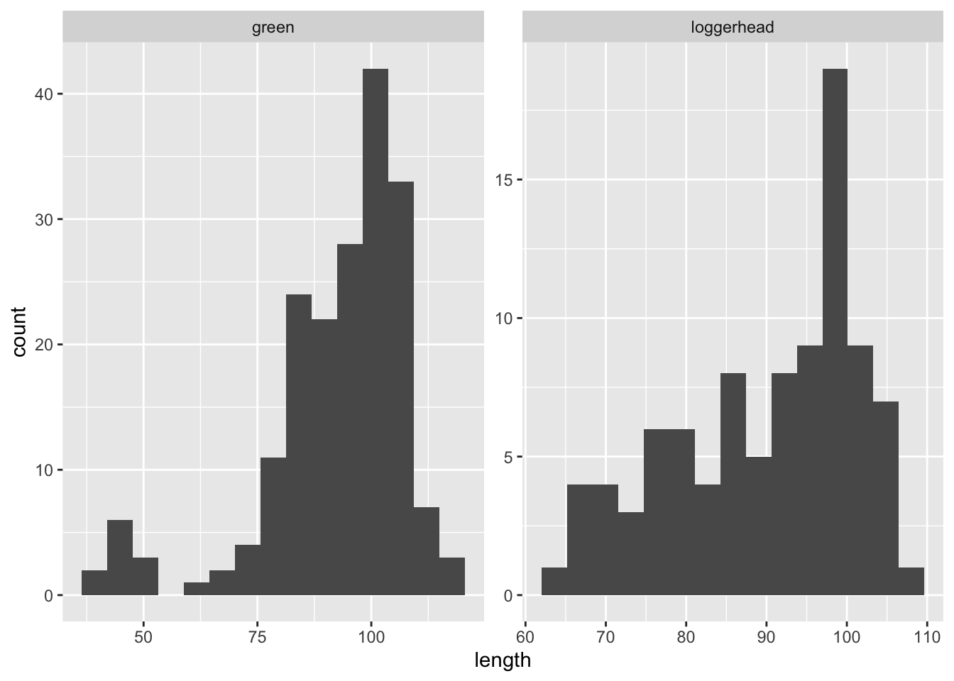
# QQ Plots
ggplot(data= sea_turtles_clean, aes(sample = length)) +
  geom_qq() +
  facet_wrap(~species)
Warning: Removed 1 rows containing non-finite values (stat_qq).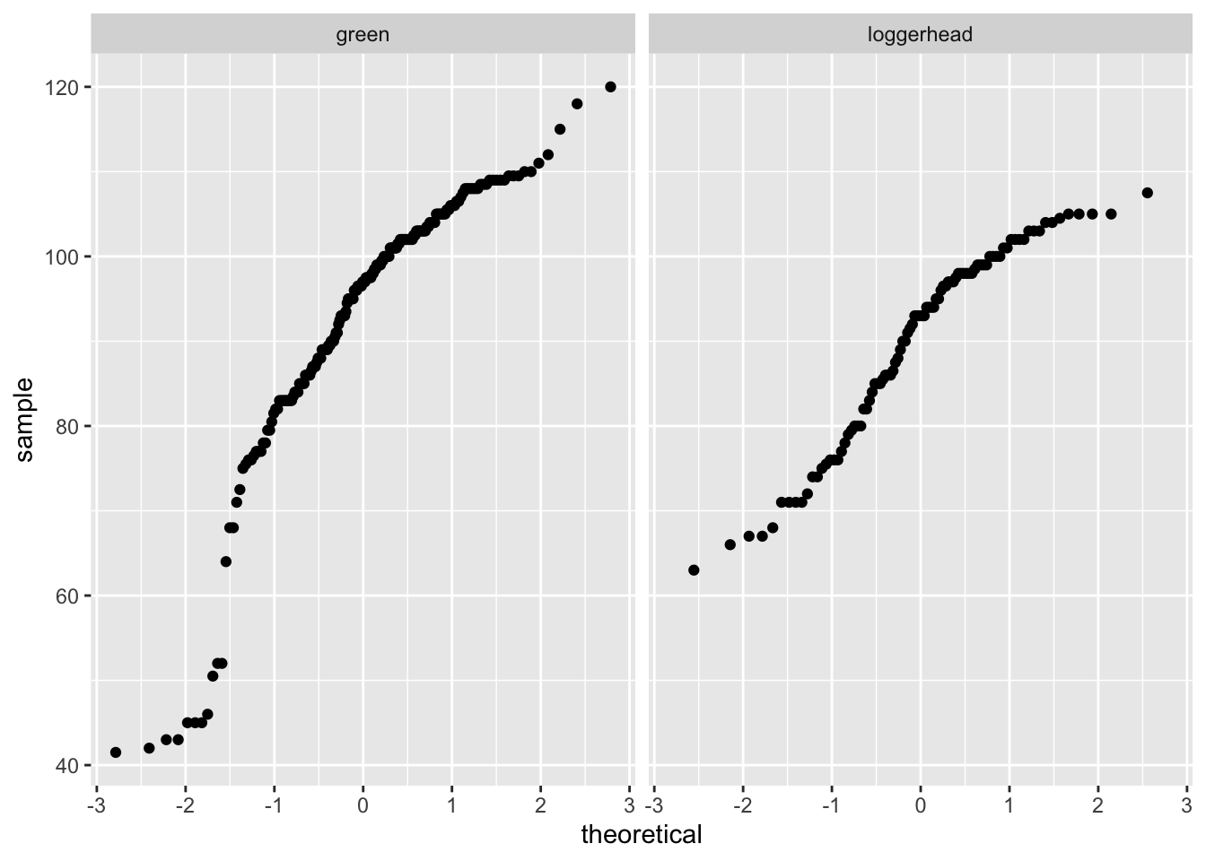
Two sample t-test
# two sample t-test
turtle_length_green <- sea_turtles_clean %>%
  dplyr::select(c("length", "species")) %>%
  filter(species == "green") %>%
  pull(length)

turtle_length_loggerhead<- sea_turtles_clean %>%
  dplyr::select(c("length", "species")) %>%
  filter(species == "loggerhead") %>%
  pull(length)

ttest <-t.test(turtle_length_green, turtle_length_loggerhead)
ttest_tidy <- tidy(ttest)

#turtles_clean_table <- sea_turtles_clean %>%
#group_by(species) %>%
  #summarise(mean_length = mean(length, na.rm=T),
            #sd_length = sd(length, na.rm=T),
            #n = n())

# cohens d/ effect size
cohen_test <- cohen.d(turtle_length_green, turtle_length_loggerhead, na.rm = TRUE)
Two sample t-test conclusions:
- I used a two-sample t-test because I wanted to compare differences between 2 groups (turtle species) and compare means (continuous data) of curved carapace lengths.
- This analysis indicates green sea turtles had a larger mean (92.64 ± 15.78, n = 188; mean ± 1 standard deviation), compares to loggerhead sea turtles which had a smaller mean (89.92 ± 11.44, n = 95; mean ± 1 standard deviation). The actual difference in means from green and loggerhead sea turtles is 2.72. The outcome of the two sample t-test indicated that there is somewhat strong chance of (p > 0.001) of randomly selecting two samples from populations with the same that are this difference by change. In sum, the difference in means is significant (Welch’s two-sample t-test: t(244.17) = 1.65, p-value = 9.98e-02) and the effect size is negligible (Cohen’s d = 0.19).
## Finalized table that shows counts and proportions of presence of burrowing barnacles to sea turtle species"
sea_turtles_burr <- sea_turtles_clean %>%
  dplyr::select(species, burr)

burr_counts <- sea_turtles_burr %>%
  janitor::tabyl(species, burr)

burr_proportions <- burr_counts %>%
  adorn_percentages() %>%
  janitor::adorn_pct_formatting(digits = 2) %>%
  adorn_ns() %>%
  drop_na()

burr_ct <- burr_proportions %>%
  column_to_rownames(var = "species")

burr_ct %>%
  kable(col.names = c("No",
                      "Yes"),
    caption = "**Table 1**: Association between sea turtle species and presence of burrowing barnacles") %>%
kable_styling(full_width = FALSE)| No | Yes | |
|---|---|---|
| green | 87.23% (164) | 12.77% (24) |
| loggerhead | 69.47% (66) | 30.53% (29) |
Chi-square test for independence
## Chi-square test
burr_ct <- burr_counts %>%
  drop_na() %>%
  column_to_rownames(var = "species")

survey_x2 <- chisq.test(burr_ct)
survey_x2
    Pearson's Chi-squared test with Yates' continuity correction

data:  burr_ct
X-squared = 11.938, df = 1, p-value = 0.00055
survey_tidy <- tidy(survey_x2)Chi-square results and summary
A chi-square test for independence compares two variables in a contingency table to see if they are related. In a more general sense, it tests to see whether distributions of categorical variables differ from each another. For this analysis, there is a significant association (i.e. non-independence) between sea turtle species and and the presence of burrowing barnacles (\(\chi\)2(1) = 11.94, p-value = 5.5e-04).
Sea turtle data source:
- Heithaus, M. and J. Thomson. 2019. Marine turtles captured during haphazard at-sea surveys in Shark Bay, Australia from February 2008 to December 2013 ver 4. Environmental Data Initiative. https://doi.org/10.6073/pasta/7696e20214fbf84f25d664ff7dc8050c