library(tidyverse)
library(deSolve)
library(here)To access .qmd script :
- the diffusion R script can be found in the folder of this repo
Load packages
R implementation
source(here("posts/2021-05-04-diffusion/R","diffusion.R"))

# run our diffusion model (iterative difference equation) with initial concentration of 10, for 8 timestep (size 1m), and 10 space steps (size 1s)
# using diffusion parameters 0.5 s/m2, 10 m2
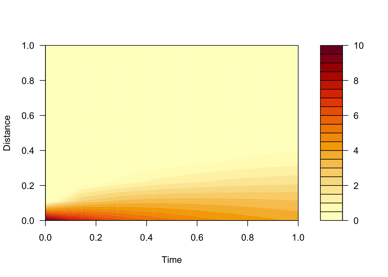
result = diff1(initialC=10, nx=10, dx=1, nt=8, dt=1, D=0.5, area=10)

# a list is returned with our 3 data frames for concentration (conc), qin and qout
# result

# used filled contour to plot results
# head(result$conc)
filled.contour(result$conc, xlab="Time", ylab="Distance")
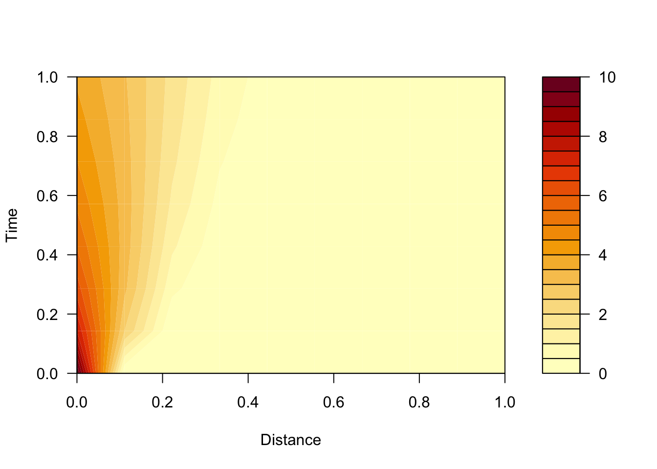
# or if you prefer this orientation (Distance on x axis)
filled.contour(t(result$conc), ylab="Time", xlab="Distance")
Change parameters (diffusivity D, and space and time steps (dx, dt))
# changes diffusivity and other parameters particularly
# diffusivity, dx and dt
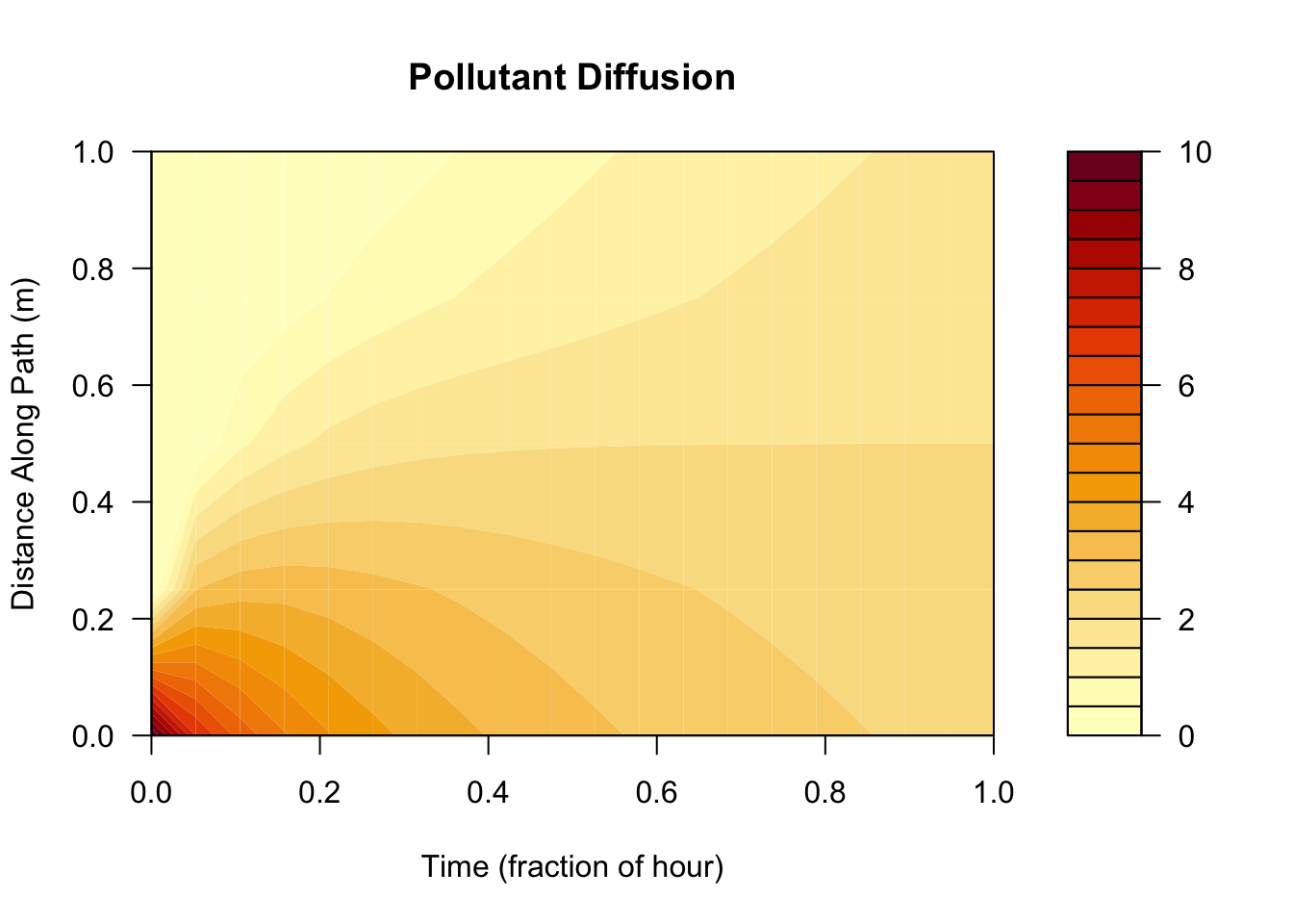
res=diff1(initialC=10,nx=5,dx=25,nt=20,dt=20,D=0.75,area=10)

filled.contour(res$conc, xlab="Time (fraction of hour)",ylab="Distance Along Path (m)", main="Pollutant Diffusion")
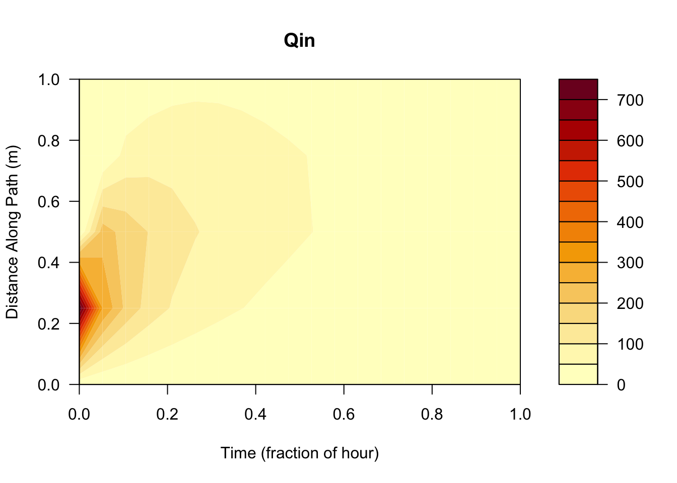
# we can also see how much material moved from place to place each time step
filled.contour(res$qin, xlab="Time (fraction of hour)",ylab="Distance Along Path (m)", main = "Qin")
Summary
we can see an overall increase in total simulation time (nt * dt) which lead to an increase in the pollutant over time and space. However, decreasing the number of discrete segments (m) lead to greater distance of the pollutant along the path.