About

Bigfoot Field Researchers Organization (BFRO) organizes and reports observations and directs expeditions to places where the observations have occurred. The overall mission of the BFRO is multifaceted, but the organization essentially seeks to resolve the mystery surrounding the bigfoot phenomenon, that is, to derive conclusive documentation of the species’ existence. This goal is pursued through the proactive collection of empirical data and physical evidence from the field and by means of activities designed to promote an awareness and understanding of the nature and origin of the evidence. See more information about the organization here.

Load packages

library(tidyverse)
library(lubridate)
library(sf)
library(here)
library(readr)
library(tidyr)
library(tigris)
library(rmapshaper)
library(mapview)

Load in Bigfoot sightings data

bigfoot_raw <- readr::read_csv(here("posts", "2024-03-15-bigfoot-exploration", "bfro_reports_geocoded.csv")) |> 
  dplyr::select(county, state, latitude, longitude, date) |> 
  tidyr::drop_na() |> 
  mutate(year = year(date)) |> 
  filter(!state %in% c("Alaska", "Hawaii"),
         !county %in% c("Idaho County", "Cowlitz County", "Flathead County")) # drop these random counties that are spatially incorrect

head(bigfoot_raw)

# A tibble: 6 × 6
  county            state         latitude longitude date        year
  <chr>             <chr>            <dbl>     <dbl> <date>     <dbl>
1 Wyoming County    West Virginia     37.6     -81.3 2005-12-03  2005
2 Windsor County    Vermont           43.5     -72.7 2005-10-08  2005
3 Wythe County      Virginia          37.2     -81.1 1984-04-08  1984
4 Wood County       Texas             32.8     -95.5 1996-12-22  1996
5 Washington County Rhode Island      41.4     -71.5 1974-09-20  1974
6 Washita County    Oklahoma          35.3     -99.2 1973-09-28  1973

Make lat and long spatial features and summarize

# Define the coordinate reference system (CRS)
crs <- st_crs(4326)

# Convert to an sf object
bigfoot_sf <- bigfoot_raw |> 
  st_as_sf(coords = c("longitude", "latitude"), 
           crs = crs) 

# Summarize the sightings by county
bigfoot_summary_df <- bigfoot_sf |>
  group_by(county) |> 
  summarise(number_of_sightings = n()) |> 
  ungroup()

Add conus sf for plotting

conus_sf <- tigris::states(cb = TRUE) |> 
  st_transform(crs) |> 
  mutate(group = case_when(
    STUSPS %in% c(state.abb[!state.abb %in% c('AK', 'HI')], 'DC') ~ 'CONUS',
    STUSPS %in% c('GU', 'MP') ~ 'GU_MP',
    STUSPS %in% c('PR', 'VI') ~ 'PR_VI',
    TRUE ~ STUSPS
    )) |>
  filter(group %in% c('CONUS')) |> 
  rmapshaper::ms_simplify(keep = 0.2)

counties_conus_sf <-tigris::counties() |> 
  st_transform(crs = crs) |> 
  left_join(conus_sf |>
              st_drop_geometry() |>
              dplyr::select(STUSPS, STATE_NAME = NAME, STATEFP, group),
                         by = 'STATEFP') |> 
  rmapshaper::ms_simplify(keep = 0.2) |> 
  st_intersection(st_union(conus_sf)) |> 
  rename(county = NAMELSAD)

Quick plot of data points

counties_outline_col = "grey80"
conus_outline_col = 'grey50'

ggplot()  +
  geom_sf(data = conus_sf,
            fill = NA,
            color  = conus_outline_col ,
            linewidth = 0.2,
            linetype = "solid") +
   geom_sf(data = counties_conus_sf,
            fill = NA,
            color  = counties_outline_col ,
            linewidth = 0.05,
            linetype = "solid") +
    geom_sf(data = bigfoot_sf,
          color = "darkgreen",
          size = 2,
          alpha = 0.5) + 
   theme_void()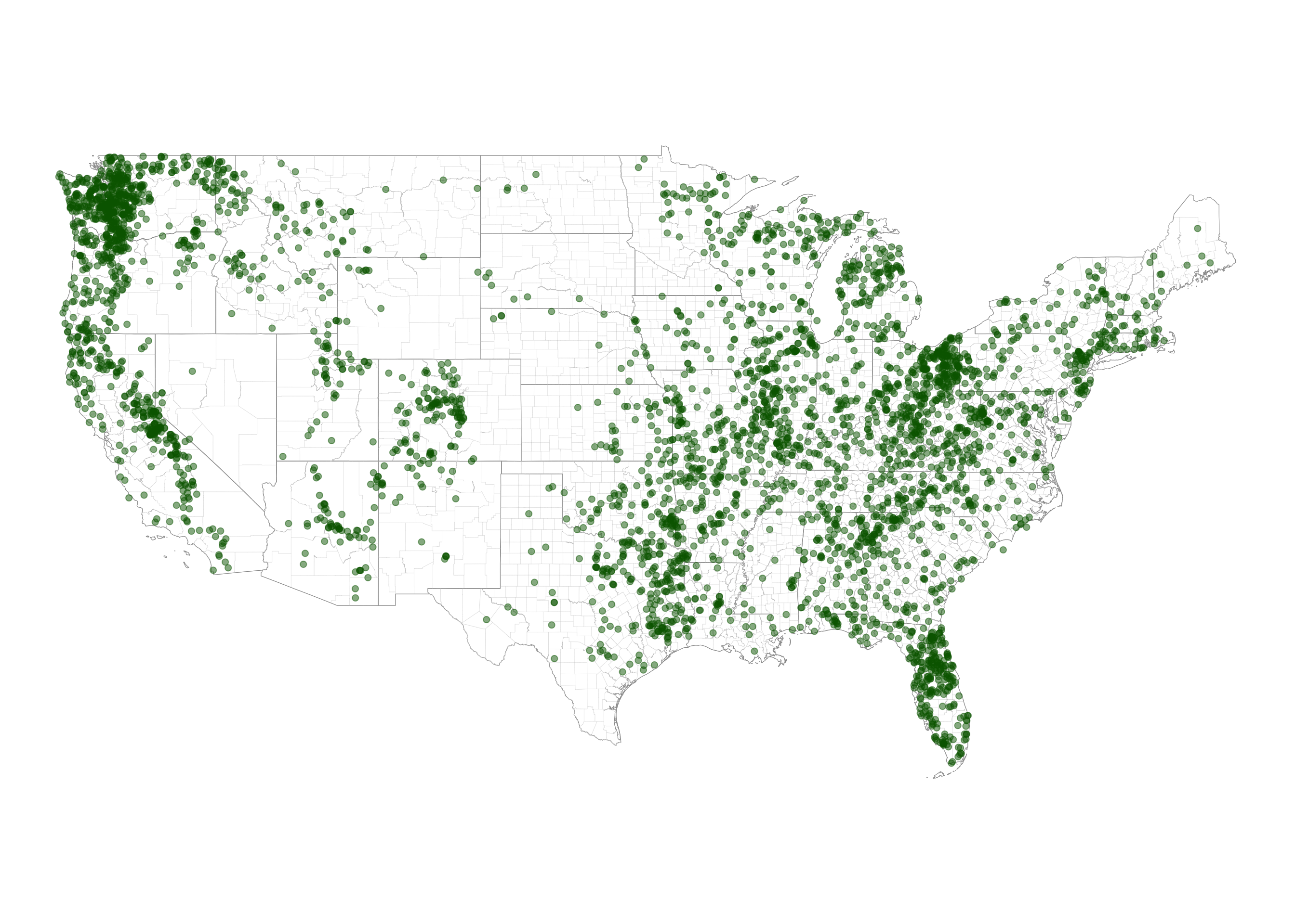

**Figure 1.** Bigfoot Sightings from 1869-2023

Interactive view of Bigfoot sightings

mapview::mapview(bigfoot_sf, alpha = 0.5, col.regions ="darkgreen",
                 layer.name = "Bigfoot Sightings from 1869-2023",
                 map.types = c("CartoDB.DarkMatter", "Esri.WorldImagery"))