About

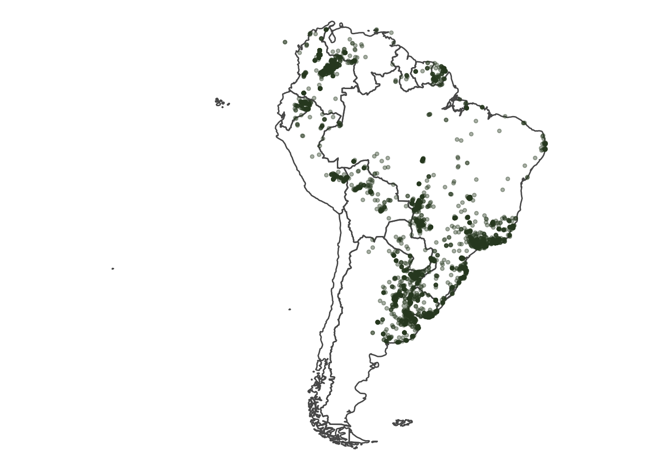
Global Biodiversity Information Facility (GBIF) is an international network and data infrastructure aimed at providing open access to biodiversity data. It serves as a global database for collecting, sharing, and disseminating biodiversity information from around the world. Here I will quickly demo how you can visualize Capybara data from GBIF across Southern America. Capybaras are the world’s largest rodents, with their closest relatives including guinea pigs! These rodents are native to South America and can weigh up to 150 lbs and grow to ~4 ft long. Capybaras grazing helps regulate plant growth in wetland environments since they are herbivores, primarily eating grasses, aquatic plants, and fruit.

Load packages

library(tidyverse)
library(tidyr)
library(sf)
library(countrycode)
library(rnaturalearth)
library(rnaturalearthdata)
library(ggspatial)

Read in raw data from Global Biodiversity Information Facilit (GBIF): https://www.gbif.org/species/search

capy_raw <- readr::read_delim("08162024-GBIF-capybara-data.csv", delim = "\t") |> 
  janitor::clean_names()

# select columns of interest
capy_sel <- capy_raw |>
  mutate(country_name = countrycode(country_code, origin = 'iso2c', destination = 'country.name')) |> 
  dplyr::select(species, country_name, decimal_latitude,
                decimal_longitude, event_date, basis_of_record) |>
  # drop NA to create sf object 
  drop_na(decimal_latitude, decimal_longitude)

Make lat and long spatial features

capy_sf <- st_as_sf(capy_sel, 
                    coords = c("decimal_longitude", "decimal_latitude"), 
                    crs = 4326)

Load in South America map

south_america <- ne_countries(scale = "medium", continent = "South America", returnclass = "sf")

Create basic ggplot map

ggplot(data = capy_sf) +
  geom_sf(data = south_america, 
          fill = NA,
          linewidth = 0.5,
          linetype = "solid") + 
  geom_sf(color = "#304529", size = 1, alpha = 0.4) +
  coord_sf(crs = 4326) +
  theme_void()

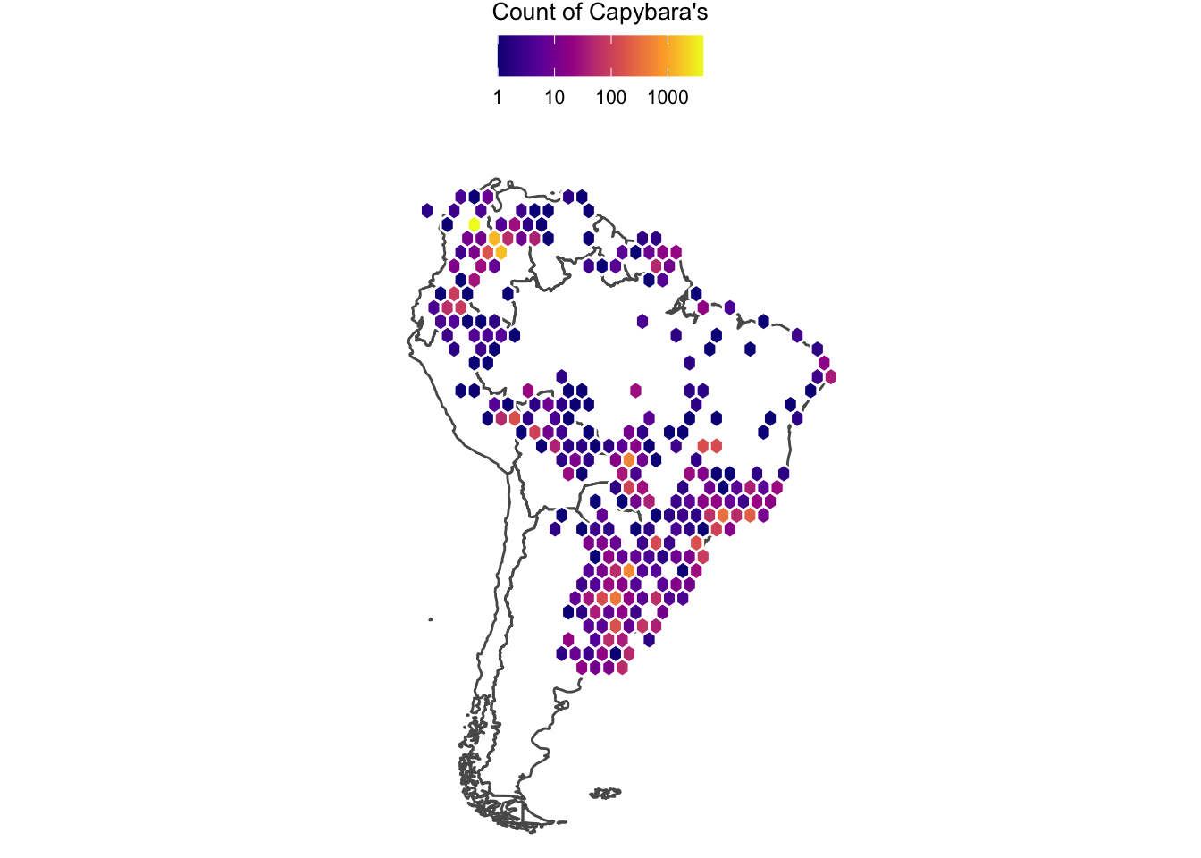
Create hexbin map with log scale

ggplot() +
  geom_sf(data = south_america, 
          fill = NA,
          linewidth = 0.5,
          linetype = "solid") +
  stat_bin_hex(data = st_coordinates(capy_sf), aes(x = X, y = Y), bins = 30, color = "white") +
  scale_fill_viridis_c(
    option = "plasma", 
    trans = "log10", 
    name = "Count of Capybara's",  
    guide = guide_colorbar(title.position = "top", title.hjust = 0.5)  
  ) +
  coord_sf(xlim = c(-85, -35), ylim = c(-55, 15), crs = 4326) +  
  theme_void() +
  theme(
    legend.position = "top",                
    legend.direction = "horizontal",        
    legend.title = element_text(size = 10), 
    legend.text = element_text(size = 8)    
  )

Interactive view of Capybara sightings in South America

# interactive view
mapview::mapview(capy_sf, alpha = 0.5, col.regions ="#4a6741", cex = 3,
                 map.types = c("CartoDB.Positron"))